Introduction

The future trend of the road surface temperature is of great importance for road maintenance. In the case of an imminent ice hazard countermeasures must be initiated well before the actual build-up of ice on the road. That is why road maintenance must be provided with detailed forecasts of all the influences on the road condition. To reach this goal, different methods can be chosen. The forecast model HS4Cast (Hertl and Schaffar, 1993) favours local measurements and locally computed forecasts of these measurements over data which are provided by a Weather Centre. This does not mean, however, that data from Weather Centres cannot be utilised by HS4Cast at all. Particularly information on precipitation can only be provided by Met offices because precipitation can never be forecast using only local measurements. So HS4Cast also benefits from the existence of Met data.

Because of the emphasis of local measurements, HS4Cast can also be used for locations where only local data are available. The model uses all major influences on the road temperature and therefore also produces forecasts of other relevant parameters like air temperature or irradiation. The basic idea of HS4Cast has been to determine all major influences on the road surface temperature and to forecast them individually before attempting to forecast the temperature of the road surface. The future road temperature is computed by solving a one-dimensional equation of heat conduction where the upper boundary condition contains the forecasts of all influencing parameters.

Different techniques are used to forecast different parameters. For some parameters, a simple extrapolation is sufficient whereas for other parameters (the majority of parameters, admittedly) more complex algorithms must be used. The recent developments for HS4Cast were directed to further improve the quality of air temperature and radiation forecasts. This has been accomplished by introducing an additional forecast engine using fuzzy logic and data bases. The paper will present these developments briefly.

Another area of interest for the user of road weather forecast systems is the possibility to compare the quality of the various models with standardised means. Until now there is no satisfying way to compare the results of different forecast systems. Yet we will try to compare the forecast quality of different models presented in recent publications.

Fuzzy logic
for the prediction
of meteoro-logical quantities

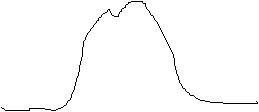
For each measurement site, "typical" patterns of meteorological parameters are maintained. For instance, three typical patterns of the irradiation for a specific site may look like this:

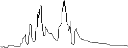
Using the rules of fuzzy logic, the actual measurements of a day are composed by such typical patterns. For the irradiation, this may look like the following combination:

	=
The actual measurements	can be seen as a mix of	85 % clear sky and	15% scattered.

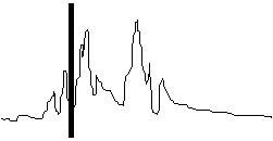
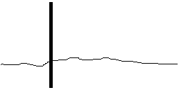
Of course, the classification cannot only be done after the data of a complete day are available; there must be a means of "on-line classification" which makes forecasts of meteorological data possible throughout the day. At the end of each day, the typical patterns of the meteorological parameters are refreshed. This brings about a continuous learning potential of the forecast engine. The following example illustrates the computation of actual forecasts, again using irradiation data:

present measurements	the future will be clear sky	the future will be scattered	the future will be overcast	the future as forecast
Analysis: 30%clear sky and 70% scattered	30% +	70% +	0%   =	the actual forecast

The use of fuzzy logic has improved the forecast quality of certain meteorological parameters, especially of radiation data and the air temperature. Furthermore, we are currently assessing the possibility of the synthesis of a road temperature forecast without solving the equation of heat conduction at all.

Comparison of forecast errors for various models

For the user of a road temperature forecast model it is of great interest to compare different methods and their outcome. It seems to be very hard to compare published statistics since every group uses different measures. We have tried to set up a list for the standard deviations of a three-hour forecast as published by various authors:

Of course, the standard deviation is not sufficient to describe the quality of a forecast completely. Moreover, it is not quite clear if all authors use the same primary data before computing statistical data. For example, it is justifiable to select only temperature data in the range between -5 and +3 °C, for instance. So it is of great importance to compare statistics of different authors with care. In many cases, unfortunately, it will not be possible at all to find equivalent statistical measures when comparing different models.

We think that it would be helpful to the end users of comparable forecast models to publish the following statistical data for the difference between the forecast (fc) and the observed (obs) (or measured) value(s) of some parameter T:

	standard deviation, sometimes also denoted as r.m.s. error
	bias (mean value)
	median absolute error

The median absolute error is defined as the median of the absolute differences between and when there are i=1,¼ ,N pairs of forecasts and measurements.

One must not mix up the above median absolute error with the mean absolute deviation or average deviation, which is defined by:

The advantage of the median absolute error is that the end user can quickly estimate the error using an obvious test: 50% of all forecasts are within the range ± (median absolute error).

It is also very interesting to figure out the hourly dependence of bias and standard deviation, as it has been done, for example, by Thornes and Shao (1992). Furthermore, a frequency distribution of the differences between actual measurements and forecasts can be done with various kinds of forecasts, for example the minimum temperature forecast or a prognosis for a specified forecast length, say three or six hours.

Bias, standard deviation, median absolute error

For the prediction of the road surface temperature three hours in advance, HS4Cast showed the following statistics for the site Hochstraß at the A21 near Vienna (536 m above sea level):

Similar results were obtained for the site Alland at the A21, which is about 14 km to the south east of Hochstraß at a height of 368 m:

If desired, HS4Cast computes forecasts very often, e.g. whenever new measurement data arrive. At the A21 there are five measurement stations (Hertl and Schaffar, 1994) and new data are delivered every two minutes. A new forecast is computed every four minutes for each outstation. It is possible to expand the forecast interval to about 15 to 20 minutes. To guarantee a sufficiently fast reaction time (HS4Cast does not rely on external forecasts!), at least four forecasts should be computed per hour. It is not necessary to compute a forecast every time when new measurement data are available.

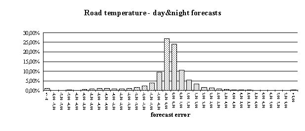
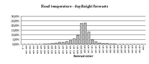
Error frequency distributions

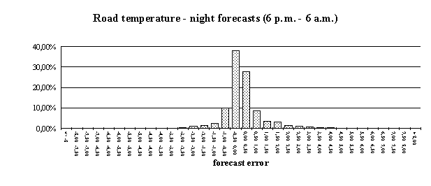
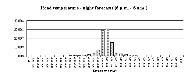
Users of forecast systems are curious to get information on the conduct of the system they bought. Graphic presentations often do a better job than plain numbers. The error frequency distribution of the forecast model in use helps to gain a better understanding of the forecasting process. The following figures demonstrate error frequency distributions for the sites Hochstraß and Alland. We decided to distribute the forecast errors (i.e. differences between forecasts and corresponding measurements) into temperature classes ranging from -8 °C to +8 °C in steps of 0.5 °C. The outermost bars belong to forecast errors which are smaller than -8 and larger than +8 °C, respectively.

Figure 1. Error distribution of three-hour forecast for site Hochstraß (Dec.1995).

Figure 2. Error distribution of three-hour forecast for site Alland (Dec.1995).

If only night-time data are considered, the errors are substantially smaller:

Figure 3. Error distribution of three-hour forecast for site Hochstraß (Dec.1995).

Figure 4. Error distribution of three-hour forecast for site Alland (Dec.1995).

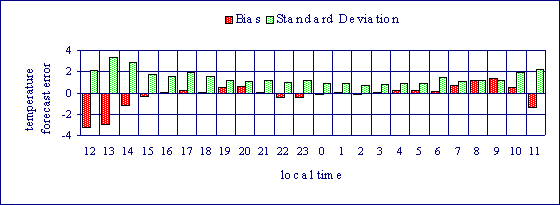
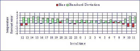
Hourly dependence of bias and standard deviation

The above numbers and diagrams tell something about the overall quality of the forecasts obtained during a particular period, for example one month. Nevertheless, the forecast errors show daily patterns. Fortunately – due to the lack of solar radiation during night-time – the errors are significantly smaller during night-time, when the risk of ice is greatest. The following figures show the hourly variation of bias and standard deviation of the three hour road temperature forecast. It can be clearly seen that the errors are smallest during the time of high risk of ice.

Figure 5. Hourly statistics for site Hochstraß in Jan.1995.

Figure 6. Hourly statistics for site Alland in Jan.1995.

Forecasts of the meteorologists

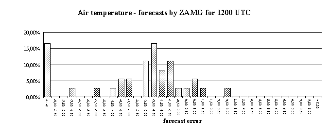
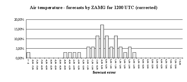
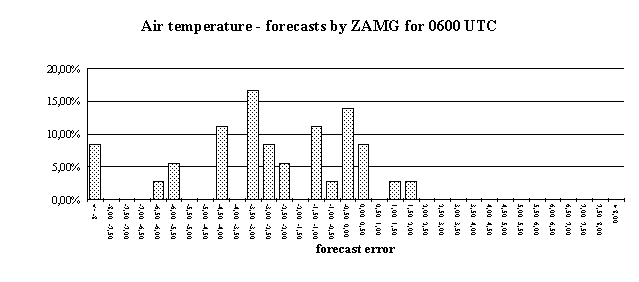
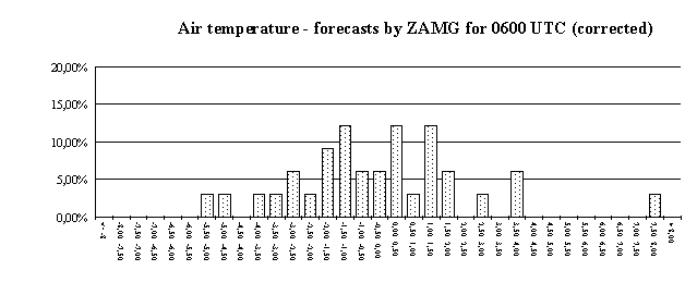
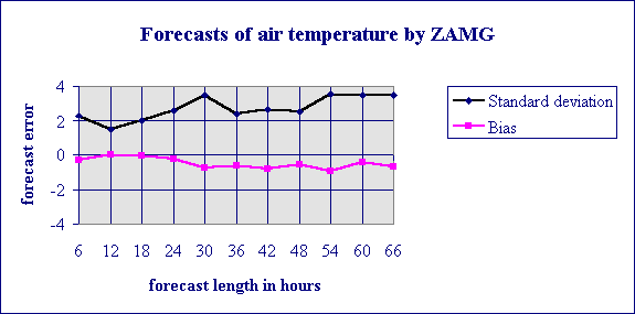
Until now, HS4Cast predicts meteorological parameters with a maximum forecast time of only three hours. For longer time horizons, the Vienna based Central Institute for Meteorology and Geodynamics (ZAMG) provides Synop weather data for the site Hochstraß which contain forecasts for up to three days. The data package includes forecasts of the air temperature, wind speed and direction, precipitation, and amount of clouds. However, the data points are not very dense: there are only forecasts for 0600 UTC, 1200 UTC, 1800 UTC and so forth.

These forecasts are provided for Hochstraß every day at 7 a.m. (0600 UTC) at the latest. So the data for 1200 UTC can be regarded as 6-hour forecasts of data to be measured at 1 p.m. The 1800 UTC forecasts will be measured at 7 p.m. and so on. (Actually, the ZAMG forecasts are computed earlier than at 0600 UTC, so the forecasts for 1200 UTC are in fact 9 to 11 hour forecasts, but from the user perspective they may be regarded as 6-hour forecasts.)

We applied the same statistics for the ZAMG forecasts as we did for HS4Cast data. It must be kept in mind, that the ZAMG forecasts for a particular prediction time are always for the same time of day, whereas HS4Cast predictions contain data for numerous times of the day. So the 6-hour ZAMG forecasts, for instance, will always be compared with data measured at 1 p.m. Moreover, there are only four forecasts for each day whereas HS4Cast computes 360 forecasts per day for each measurement site at the A21.

The following diagrams show some error distributions for ZAMG forecasts of the air temperature. The figures contain data from late November 1995 until mid-January 1996. It can be clearly seen that the bias can be reduced considerably if the difference between the first ZAMG forecast (this is the forecast for 0600 UTC) and the corresponding measurement is computed to correct the offset in the forecasts. Of course, this indicates that external temperature forecasts are of questionable value if no measurements are taken to correct the inherent bias. For predictions of the amount of clouds no such bias has to be considered.

Figure 7. Error distribution of six-hour forecast for site Hochstraß (produced by ZAMG).

Figure 8. Error distribution of six-hour forecast for site Hochstraß (produced by ZAMG, corrected by eliminating bias of 0600 UTC forecast for the same day).

Figure 9. Error distribution of 24-hour forecast for site Hochstraß (produced by ZAMG).

Figure 10. Error distribution of 24-hour forecast for site Hochstraß (produced by ZAMG, corrected by eliminating bias of 0600 UTC forecast for the previous day).

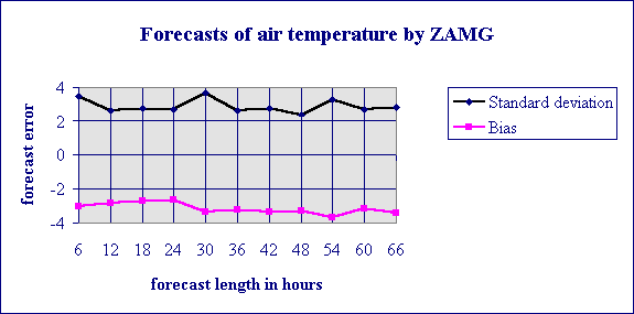
A comprehensive analysis of the forecast errors of the ZAMG predictions shows that there is no great loss in accuracy if predictions with longer forecast length are taken. The following two diagrams, where the forecast errors are shown as functions of forecast length, reveal this in greater detail. Again, the numbers are valid for the prediction of the air temperature.

Figure 11. Errors of ZAMG forecasts without elimination of bias.

Figure 12. Errors of corrected ZAMG forecasts.

The standard deviations of the six-, 30- and 54-hour forecasts are higher than the values for adjacent forecast lengths. Since these forecasts are predictions for 1 p.m. this behaviour may indicate that also for meteorologists it is harder to forecast temperatures for times around noon than for night-times. In other words, also the forecasts of the meteorologists probably contain an hourly dependence similar to the behaviour shown in Figures 5 and 6.

References

A.Basile, F.Butini and R.Selvi (1994), Air temperature nowcasting up to three hours along Italian motorway using artificial neural networks, Proceedings of SIRWEC 1994: 29

J.Bogren and T.Gustavsson (1994), A Combined Statistical and Energy Balance Model for Prediction of Road Surface Temperature, Proceedings of SIRWEC 1994: 43

P.W.Fröhling (1994), A Neural Network for Short Term Temperature Forecast on Roads, Proceedings of the IXth PIARC International Winter Road Congress: 601

S.Hahn (1994), Straßenzustands- und Wetter-Informationssystem in der Bundesrepublik Deutschland (SWIS), Proceedings of the IXth PIARC International Winter Road Congress: 16

S.Hertl and G.Schaffar (1993), The Prediction of Ice on Roads, Proceedings of the Twelfth IASTED International Conference, MODELLING, IDENTIFICATION AND CONTROL: 54

S.Hertl and G.Schaffar (1994), Are local measurements needed for the prediction of ice on roads?, Proceedings of SIRWEC 1994: 221

S.Hertl and G. Schaffar (1995), The Prediction of Ice on Roads Using Fuzzy-Logic, Proceedings of the 28th International Symposium on Automotive Technology and Automation (Advanced Transportation Systems): 401

B.H.Sass and H.Voldborg (1994), On the operational use of a numerical model for prediction of road temperature and ice, Proceedings of SIRWEC 1994: 1

J.E.Thornes and J.Shao (1992), Meteorological Magazine, 121: 197